Maths Unit 1 ( Theory )

 -------------------  Introduction and history of data science------------------------------------

Introduction to Data Science:

Data Science is an interdisciplinary field that involves extracting insights and knowledge from structured and unstructured data. It combines various disciplines such as statistics, mathematics, computer science, and domain knowledge to analyze and interpret data, uncover patterns, make predictions, and drive data-driven decision-making.

Data scientists use a combination of techniques, tools, and algorithms to collect, clean, transform, and analyze large volumes of data. They apply statistical modeling, machine learning, data visualization, and other analytical methods to extract valuable information from data and generate actionable insights.

History of Data Science:

The roots of Data Science can be traced back to several disciplines and technological advancements over the years. Here is a brief history of some key milestones:

1. Statistics and Mathematics:

- The development of statistical methods in the early 20th century, pioneered by statisticians like Ronald Fisher and Karl Pearson, laid the foundation for data analysis and inference.

- Mathematical concepts such as linear algebra, calculus, and probability theory provide the fundamental principles for statistical modeling and machine learning algorithms used in Data Science.

2. Information Theory:

- In the 1940s, Claude Shannon introduced information theory, which focused on quantifying and transmitting information efficiently. This theory became essential for understanding data storage, compression, and transmission.

3. Computing and Data Storage:

- The advent of computers and advancements in data storage technologies facilitated the handling of large datasets.

- In the 1960s and 1970s, the development of databases and data management systems provided efficient storage and retrieval mechanisms for data.

4. Data Mining and Machine Learning:

- In the late 1980s and early 1990s, the term "Data Mining" emerged, focusing on the automatic extraction of patterns and knowledge from large datasets.

- Machine learning techniques gained popularity, with algorithms like decision trees, neural networks, and support vector machines being developed.

5. Big Data and Web 2.0:

- The rise of the internet and the emergence of Web 2.0 platforms in the early 2000s generated massive amounts of data from various online sources, such as social media, e-commerce, and sensors.

- The term "Big Data" gained prominence, highlighting the need for new tools and techniques to handle, process, and analyze vast volumes of data.

6. Data Science as a Field:

- Around the mid-2000s, Data Science began to emerge as a distinct field, driven by the convergence of statistics, machine learning, computer science, and domain expertise.

- The availability of powerful computational resources, open-source software frameworks, and increased data accessibility further propelled the growth of Data Science.

Real-Life Examples:

Data Science has made a significant impact across various industries and domains. Here are a few real-life examples:

1. Healthcare:

- Data Science is used in healthcare to analyze patient data, identify disease patterns, predict patient outcomes, and personalize treatments.

- For example, data analysis techniques can help identify risk factors for certain diseases, optimize treatment plans, or predict patient readmissions.

2. Finance:

- In the finance industry, Data Science is utilized for fraud detection, credit risk assessment, algorithmic trading, and portfolio optimization.

- For instance, machine learning algorithms can be used to detect unusual patterns in financial transactions, flagging potential fraudulent activities.

3. E-commerce and Marketing:

- Data Science plays a crucial role in e-commerce and marketing by analyzing customer behavior, recommending products, and optimizing marketing campaigns.

- Recommendation systems, powered by machine learning algorithms, provide personalized product suggestions based on customer browsing and purchase history.

4. Transportation and Logistics:

- Data Science is employed in transportation and logistics to optimize routes, predict demand, and enhance supply chain operations.

- For example, predictive analytics can help determine the most efficient routes for delivery vehicles, considering factors

 like traffic conditions and delivery time windows.

5. Social Media and Sentiment Analysis:

- Data Science techniques are utilized to analyze social media data, understand user sentiments, and extract valuable insights.

- Sentiment analysis algorithms can process large volumes of social media posts to determine public opinion about a product, service, or event.

These examples illustrate how Data Science has become an integral part of various industries, driving innovation, improving decision-making, and creating value from data.

---------------------------------------Introduction and history of machine learning----------------------------

Introduction to Machine Learning:

Machine Learning (ML) is a subfield of Artificial Intelligence (AI) that focuses on the development of algorithms and models that enable computers to learn from and make predictions or decisions based on data, without being explicitly programmed. The core idea behind machine learning is to allow machines to learn from patterns and experiences to improve their performance on a specific task.

In machine learning, models are trained on historical data, called training data, and then used to make predictions or take actions on new, unseen data. The process involves identifying patterns, relationships, and trends within the data, which the machine learning algorithms use to generalize and make predictions on new instances.

Machine learning can be categorized into three main types:

1. Supervised Learning: In supervised learning, the model is trained on labeled data, where the input data is associated with corresponding labels or target values. The model learns to map the input to the correct output based on the provided examples. It can then make predictions on new, unlabeled data by generalizing from the training data.

2. Unsupervised Learning: Unsupervised learning deals with unlabeled data. The model aims to find hidden patterns, structures, or relationships within the data without any pre-existing knowledge of the output. Clustering and dimensionality reduction are common tasks in unsupervised learning.

3. Reinforcement Learning: Reinforcement learning involves an agent interacting with an environment to learn a sequence of actions that maximize a reward signal. The agent learns through trial and error, receiving feedback in the form of rewards or penalties for its actions. The goal is to find an optimal policy that maximizes the cumulative reward over time.

History of Machine Learning:

The history of machine learning can be traced back to the mid-20th century, with significant contributions from various fields. Here are some key milestones in the history of machine learning:

1. Early Concepts and Foundations:

- In the 1940s and 1950s, the foundations of machine learning were laid, with researchers like Alan Turing and Arthur Samuel exploring concepts of machine intelligence and developing early learning algorithms.

- The introduction of the perceptron algorithm by Frank Rosenblatt in 1957 marked a significant development in the field.

2. Development of Neural Networks:

- In the 1960s and 1970s, the field of neural networks emerged, inspired by the structure and function of the human brain. Researchers such as Marvin Minsky and Seymour Papert made significant contributions to neural network theory and architecture.

3. Rise of Decision Trees and Rule-Based Systems:

- In the 1980s, decision tree algorithms, such as ID3 and C4.5, gained popularity for classification tasks. Rule-based systems, like expert systems, also became prominent in capturing knowledge and making decisions.

4. Evolution of Support Vector Machines and Kernel Methods:

- In the 1990s, support vector machines (SVM) were introduced by Vladimir Vapnik and his colleagues. SVMs became widely used for both classification and regression tasks.

- Kernel methods, which enable non-linear learning in high-dimensional spaces, also gained attention during this time.

5. Advancements in Deep Learning:

- In the 2000s and onwards, deep learning witnessed significant advancements. Deep neural networks with multiple layers became feasible to train thanks to improved computational power and the availability of large-scale datasets.

- Deep learning models, such as convolutional neural networks (CNNs) for image analysis and recurrent neural networks (RNNs) for sequential data, achieved remarkable breakthroughs in areas like computer vision and natural language processing.

6. Expansion of Machine Learning Applications:

- In recent years, machine learning has expanded its application to various domains, including healthcare, finance, e-commerce, robotics, and more. The availability of vast amounts of data, increased

 computational power, and advancements in algorithms have driven this growth.

These milestones demonstrate the evolution of machine learning from its early foundations to the current era of sophisticated algorithms and widespread applications. Machine learning continues to advance, with ongoing research and developments pushing the boundaries of what is possible in AI and data-driven decision-making.

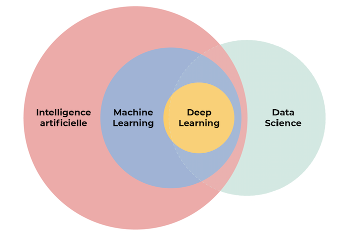
-----------------------------------Overlap between data science and machine learning --------------------

Data Science and Machine Learning share a significant overlap, as they are closely related fields that often work together to extract insights and value from data. Here are some key areas of overlap between Data Science and Machine Learning:

1. Data Preparation and Cleaning:

Both Data Science and Machine Learning require data preprocessing, which involves tasks such as data cleaning, transformation, feature engineering, and handling missing values. Data scientists and machine learning practitioners often use similar techniques to ensure data quality and prepare the data for analysis or model training.

2. Exploratory Data Analysis:

Exploratory Data Analysis (EDA) is a crucial step in both Data Science and Machine Learning workflows. It involves visualizing and understanding the data, identifying patterns, correlations, outliers, and other relevant insights. Data scientists and machine learning practitioners leverage EDA techniques to gain insights into the data and make informed decisions about feature selection, data transformation, and model building.

3. Feature Selection and Engineering:

Feature selection and engineering play a vital role in both Data Science and Machine Learning. Data scientists and machine learning practitioners identify and select the most relevant features from the data that can contribute to accurate predictions or meaningful insights. They may also engineer new features by combining or transforming existing ones to improve model performance.

4. Model Building and Evaluation:

Both Data Science and Machine Learning involve building predictive models. Data scientists and machine learning practitioners utilize various algorithms and techniques to train models on the data. They evaluate the performance of these models using metrics such as accuracy, precision, recall, and F1 score. Model selection, hyperparameter tuning, and validation techniques (e.g., cross-validation) are also common aspects shared between the two fields.

5. Predictive Analytics and Decision Making:

Both Data Science and Machine Learning aim to make predictions or inform decision-making based on data. Data scientists and machine learning practitioners use statistical modeling, regression analysis, classification algorithms, and other predictive techniques to derive insights, make accurate predictions, and drive data-driven decision-making.

6. Deployment and Productionization:

Once a model is developed, both Data Science and Machine Learning involve deploying the model into production environments. This includes integrating the model into software systems, building APIs for real-time predictions, and ensuring scalability and performance. Data scientists and machine learning practitioners collaborate to operationalize and maintain the models in real-world applications.

While there is overlap between Data Science and Machine Learning, it's important to note that Data Science encompasses a broader range of skills and tasks, including data collection, database management, data visualization, and domain expertise. Machine Learning, on the other hand, specifically focuses on developing algorithms and models to make predictions or decisions based on data.

------------------Application of machine learning and data science and artificial intelligence in the modern world context -----------------------------------

Machine Learning (ML), Data Science, and Artificial Intelligence (AI) have revolutionized numerous industries and have a wide range of applications in the modern world. Here are some key areas where ML, Data Science, and AI are being applied:

1. Healthcare:

- Disease Diagnosis and Prediction: ML models are used to analyze medical images, such as X-rays and MRI scans, for early detection and accurate diagnosis of diseases.

- Drug Discovery and Development: ML techniques help in identifying potential drug candidates, predicting drug efficacy, and optimizing treatment plans.

- Personalized Medicine: ML algorithms analyze patient data to provide tailored treatment plans and predict individual responses to medications.

2. Finance and Banking:

- Fraud Detection: ML models analyze patterns in transactions and user behavior to identify fraudulent activities, such as credit card fraud or money laundering.

- Risk Assessment: ML algorithms assess credit risk, predict stock market trends, and determine investment strategies based on historical data.

- Algorithmic Trading: ML models analyze market data and make automated trading decisions to optimize investment returns.

3. Transportation and Logistics:

- Autonomous Vehicles: ML and AI algorithms enable self-driving cars and autonomous drones to perceive the environment, navigate routes, and make decisions in real-time.

- Traffic Optimization: ML models analyze traffic patterns and historical data to optimize traffic flow, reduce congestion, and improve transportation efficiency.

- Supply Chain Management: ML techniques optimize inventory management, demand forecasting, and route optimization for efficient logistics operations.

4. Retail and E-commerce:

- Recommendation Systems: ML algorithms analyze customer preferences and behavior to provide personalized product recommendations, enhancing customer experience and increasing sales.

- Price Optimization: ML models analyze market data, competitor pricing, and customer behavior to optimize pricing strategies and maximize revenue.

- Demand Forecasting: ML algorithms predict future demand based on historical sales data, enabling retailers to optimize inventory management and supply chain operations.

5. Natural Language Processing (NLP) and Language Translation:

- Chatbots and Virtual Assistants: NLP techniques enable conversational agents to understand and respond to user queries, providing customer support and information retrieval.

- Language Translation: ML models power automatic language translation services, making communication across languages more accessible.

6. Energy and Utilities:

- Smart Grid Optimization: ML algorithms analyze energy consumption patterns and optimize energy distribution and usage for efficient grid management.

- Predictive Maintenance: ML models analyze sensor data to predict equipment failures and enable proactive maintenance, reducing downtime and improving operational efficiency.

These are just a few examples of the vast range of applications for ML, Data Science, and AI in the modern world. The potential impact of these technologies continues to grow as new advancements and innovative use cases emerge across industries.

--------------------------Types of data-------------------------------------

Types of data

--------------------------------------------------------Measure of location -----------------------------------

Measures of location, also known as measures of central tendency, are statistical metrics that provide information about the center or average value of a dataset. They summarize the typical or representative value around which the data tends to cluster. Here are some commonly used measures of location:

1. Mean: The mean, also called the arithmetic average, is calculated by summing up all the values in a dataset and dividing it by the total number of observations. It is sensitive to extreme values and provides a balanced estimate of the dataset's central value.

2. Median: The median is the middle value in an ordered dataset. To find the median, the data points are arranged in ascending or descending order, and the value that falls in the middle is selected. If there is an even number of observations, the median is the average of the two middle values. The median is less affected by extreme values and is useful when the data is skewed or contains outliers.

3. Mode: The mode represents the value or values that occur most frequently in a dataset. It is applicable to categorical or discrete data and can have multiple modes if there are multiple values with the same highest frequency. The mode is useful for identifying the most common category or value in a dataset.

4. Weighted Mean: In some cases, different data points may have different weights or importance. The weighted mean takes into account these weights when calculating the average. Each data point is multiplied by its corresponding weight, and the sum of the weighted values is divided by the sum of the weights.

These measures of location provide different perspectives on the central tendency of a dataset. The choice of measure depends on the nature of the data, the presence of outliers, and the specific objective of the analysis.

------------------------------------Measure of variabillity------------------------------------------

Measures of variability, also known as measures of dispersion, provide information about the spread or dispersion of data points in a dataset. They quantify the degree of variability or diversity within the dataset. Here are some commonly used measures of variability:

1. Range: The range is the simplest measure of variability and is calculated as the difference between the maximum and minimum values in a dataset. It gives an indication of the total spread of the data but is sensitive to extreme values.

2. Variance: Variance measures the average squared deviation of each data point from the mean. It calculates the average of the squared differences between each data point and the mean, providing a measure of how far the data points are spread out from the mean. Variance is influenced by extreme values and provides a measure of both the magnitude and direction of the deviations.

3. Standard Deviation: The standard deviation is the square root of the variance and provides a more interpretable measure of variability. It quantifies the average distance of data points from the mean. A smaller standard deviation indicates that the data points are closer to the mean, while a larger standard deviation indicates greater dispersion.

4. Interquartile Range (IQR): The IQR is a measure of the spread of data within the middle 50% of the dataset. It is calculated as the difference between the 75th percentile (third quartile) and the 25th percentile (first quartile). The IQR is less sensitive to extreme values and provides a robust measure of variability.

5. Mean Absolute Deviation (MAD): MAD calculates the average absolute deviation of each data point from the mean. It provides a measure of the average distance between each data point and the mean, regardless of the direction of deviation. MAD is less influenced by extreme values and is useful when outliers are present.

6. Coefficient of Variation (CV): CV is the ratio of the standard deviation to the mean, expressed as a percentage. It provides a relative measure of variability, allowing for comparison across datasets with different scales. A higher CV indicates greater relative variability.

These measures of variability help to understand the spread and dispersion of data points in a dataset. They provide insights into the diversity and distribution of the data and are useful for comparing datasets, identifying outliers, and assessing the reliability of statistical analyses.

----------------------------------Measure of shape --------------------------------------------------

Measures of shape, also known as measures of distribution, describe the characteristics of the shape or pattern of a dataset. They provide insights into the symmetry, skewness, and kurtosis of the data distribution. Here are some commonly used measures of shape:

1. Skewness: Skewness measures the asymmetry of a distribution. It quantifies the extent to which the data is skewed or shifted to one side. Positive skewness indicates a longer tail on the right side of the distribution, while negative skewness indicates a longer tail on the left side. Skewness helps identify departures from a symmetric distribution.

2. Kurtosis: Kurtosis measures the shape of the distribution's tails. It quantifies the degree of peakedness or flatness compared to a normal distribution. High kurtosis indicates heavy tails and a sharper peak (leptokurtic), while low kurtosis indicates lighter tails and a flatter peak (platykurtic). Kurtosis helps identify departures from the normal distribution.

3. Histogram: A histogram is a graphical representation of the distribution of a dataset. It displays the frequency or count of data points within different intervals or bins. By visualizing the histogram, you can observe the shape of the distribution, such as whether it is symmetric, skewed, or multimodal.

4. Quantile-Quantile (Q-Q) Plot: A Q-Q plot is a graphical tool used to assess if a dataset follows a specific distribution (e.g., normal distribution). It compares the quantiles of the observed data against the quantiles of the theoretical distribution. A straight line in the plot suggests a good fit to the theoretical distribution, while deviations indicate departures from the assumed shape.

5. Shapiro-Wilk Test: The Shapiro-Wilk test is a statistical test used to assess the normality of a dataset. It determines whether the data significantly deviates from a normal distribution. If the p-value obtained from the test is below a certain threshold (e.g., 0.05), it suggests a departure from normality.

These measures of shape provide insights into the characteristics of a dataset's distribution. They help identify departures from normality, assess the presence of skewness or heavy tails, and determine the appropriate statistical techniques for data analysis. Understanding the shape of the distribution is crucial for making accurate inferences and selecting appropriate statistical models.

\------------------------------Case study of Bollywood dataset ----------------------------------------

Sure! Let's consider a case study of a Bollywood dataset to demonstrate how data analysis can provide insights into the Indian film industry. In this case study, we will explore a dataset containing information about Bollywood movies, including their release year, genre, budget, box office collection, and ratings.

Objective: The objective of this case study is to analyze the Bollywood dataset to gain insights into the trends, success factors, and patterns within the industry.

Steps:

1. Data Collection: Gather data on Bollywood movies, including information such as movie title, release year, genre, budget, box office collection, and ratings. This data can be collected from various sources, such as movie databases, film industry reports, and public sources.

2. Data Cleaning and Preparation: Clean the dataset by handling missing values, removing duplicates, and formatting the data appropriately. Convert relevant columns to their respective data types (e.g., numeric, categorical) for analysis.

3. Exploratory Data Analysis (EDA):

   - Descriptive Statistics: Calculate summary statistics such as mean, median, range, and standard deviation for relevant columns (e.g., budget, box office collection) to understand the overall distribution and variability of the data.

   - Genre Analysis: Analyze the distribution of movies across different genres to identify popular genres in Bollywood and observe any changes in genre preferences over the years.

   - Budget and Box Office Analysis: Explore the relationship between movie budgets and box office collections. Identify the highest-grossing movies, examine their budget-to-collection ratios, and analyze the success factors contributing to their box office success.

   - Time Series Analysis: Examine the trend of movie releases and box office collections over the years to identify any patterns or fluctuations. Identify the years with the highest and lowest movie releases and box office revenues.

   - Rating Analysis: Analyze the distribution of movie ratings to understand the audience reception and the impact of ratings on box office performance.

4. Visualization: Create visualizations such as bar charts, line plots, histograms, and scatter plots to visually represent the insights gained from the EDA. Visualizations can help in better understanding trends, patterns, and relationships within the dataset.

5. Statistical Analysis: Conduct statistical tests and analyses, such as correlation analysis, hypothesis testing, or regression analysis, to uncover significant relationships or factors that contribute to a movie's success in terms of box office performance or ratings.

6. Insights and Recommendations: Based on the analysis, draw meaningful insights about the Bollywood industry, including popular genres, factors influencing box office success, and audience preferences. Provide recommendations for filmmakers, production houses, or distributors based on the findings to make informed decisions and improve the chances of success in the industry.

This case study showcases how data analysis can provide valuable insights into the Bollywood film industry. By analyzing the dataset, one can gain a better understanding of trends, factors influencing success, and audience preferences, enabling stakeholders to make data-driven decisions in their filmmaking endeavors.

---------------------------------------case study of cardio diseases dataset --------------------------------

Certainly! Let's consider a case study on coronary heart disease (CHD) to illustrate how data analysis can provide insights into the risk factors and potential predictors of this cardiovascular condition.

Objective: The objective of this case study is to analyze a dataset related to coronary heart disease to identify significant risk factors and explore potential predictors of CHD.

Steps:

1. Data Collection: Gather data related to coronary heart disease, including variables such as age, gender, cholesterol levels, blood pressure, body mass index (BMI), smoking habits, family history of CHD, and presence or absence of coronary heart disease. This data can be obtained from medical records, health surveys, or research studies.

2. Data Cleaning and Preparation: Clean the dataset by handling missing values, removing duplicates, and ensuring consistency in data formatting. Convert relevant variables to their appropriate data types (e.g., numeric, categorical) for analysis.

3. Exploratory Data Analysis (EDA):

   - Descriptive Statistics: Calculate summary statistics for key variables, such as mean, median, range, and standard deviation, to understand the distribution and variability of the data.

   - Univariate Analysis: Analyze individual variables to identify any trends or patterns. For example, examine the distribution of age, cholesterol levels, and blood pressure among individuals with and without CHD.

   - Bivariate Analysis: Explore the relationship between variables and CHD. Conduct statistical tests or create visualizations to examine the association between age, gender, lifestyle factors (smoking habits, BMI), and CHD prevalence.

   - Feature Selection: Use techniques such as correlation analysis or feature importance ranking to identify the most influential predictors of CHD.

   - Data Visualization: Create charts, graphs, or heatmaps to visually represent the relationships and patterns discovered during the analysis.

4. Statistical Analysis: Conduct statistical tests and analyses to investigate the significance of risk factors. For example:

   - Chi-square test or Fisher's exact test to examine the association between categorical variables (e.g., gender, smoking habits) and CHD.

   - T-test or ANOVA to compare means of continuous variables (e.g., age, cholesterol levels) between individuals with and without CHD.

   - Logistic regression to assess the relationship between multiple predictors and the presence of CHD, controlling for confounding factors.

5. Insights and Recommendations: Based on the analysis, draw meaningful insights regarding the risk factors and predictors of coronary heart disease. Identify significant variables that are associated with CHD and understand their impact on disease prevalence. Provide recommendations for healthcare providers, policymakers, or individuals to promote prevention, early detection, and management of CHD.

This case study demonstrates how data analysis can help identify significant risk factors and potential predictors of coronary heart disease. By analyzing the dataset, it is possible to gain insights into the relationships between various variables and CHD prevalence, aiding in the development of preventive measures and personalized healthcare strategies.